Excel has always been a powerhouse for organizing, analyzing, and cleaning data, but some functions truly change the game. The UNIQUE function is one of those. Introduced in modern versions of Excel, UNIQUE helps you extract distinct or one-time values instantly, without manually deleting duplicates or using complicated workarounds. Whether you’re cleaning up customer lists, generating dropdown menus, or building advanced dashboards, UNIQUE is an essential tool for modern Excel users.
This comprehensive guide walks you through everything you need to know about the UNIQUE function: how it works, key features, everyday use cases, advanced combinations with other functions, and common troubleshooting issues.
What Is the UNIQUE Function in Excel?

The UNIQUE function returns a list of distinct values from a given range. Instead of using manual tools like “Remove Duplicates,” UNIQUE dynamically generates a new list based on your original dataset, meaning it automatically updates whenever your data changes. Its syntax looks like this:
=UNIQUE(a, b, c)
Here’s what each element means:
- a (array) – The range or table from which you want to extract unique values
- b (Boolean Value) – An optional logical (TRUE/FALSE) argument. Use FALSE (default) to compare rows, or TRUE to compare columns.
- c – This is again a Boolean Value. Use TRUE if you want to extract only those values that appear exactly one time
This makes UNIQUE a versatile and dynamic tool for data management, perfect for everything from simple deduplication to complex filtering tasks.
Key Features of the UNIQUE Function in Excel

UNIQUE may look simple, but it’s packed with powerful capabilities. Here’s a deeper look at what makes it so valuable.
1. Dynamic Range Creation
UNIQUE is a dynamic array function. This means:
- It automatically spills results into adjacent cells
- It expands or contracts based on the size of your data
- You don’t need to copy formulas manually or adjust ranges
If your data grows (e.g., more customer names), the UNIQUE output updates instantly. If the data shrinks, the output shrinks too.
2. Empty Cells Requirement (Spill Behavior)
Because UNIQUE spills its result, Excel needs enough empty cells to display the output. If the spill area is blocked by any value, Excel shows a #SPILL error. Once the space is cleared, the formula will work again.
Example: If you write UNIQUE in cell C2 and C3 already contains data, Excel can’t spill.
3. Automatic Updates
UNIQUE recalculates automatically anytime:
- You add new values to the source
- You delete values
- Data inside the range changes
You never need to refresh the formula manually, making UNIQUE ideal for real-time reports.
4. Cross-Workbook Functioning
Dynamic array functions like UNIQUE can reference data from other open workbooks. However, if the source workbook is closed, the UNIQUE formula will return a #REF! error, indicating that the reference is no longer accessible.
As new rows get added to the table, UNIQUE updates automatically, no need to adjust ranges.
Using the UNIQUE Function to Remove Duplicates

The UNIQUE function in Excel is designed to extract and display distinct values from a range or list, automatically removing any duplicates. It helps you create a clean, organized dataset that is perfect for data analysis, reporting, or filtering results without redundancy.
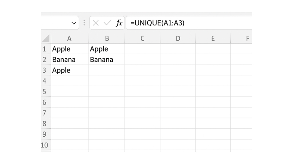
For instance, if your list contains “Apple,” “Banana,” and “Apple,” the UNIQUE function will return just “Apple” and “Banana,” showing each value once.
Here’s how to use it step-by-step:
- Step 1: Open Excel
Launch Microsoft Excel on your device.
- Step 2: Enter Data
In cell A1, type “Apple”, in A2 type “Banana”, and in A3 type “Apple.” This gives you a short list with a duplicate entry.
- Step 3: Select Output Range
Click on cell B1, where you’d like the unique values to appear.
- Step 4: Enter the Formula
Type “=UNIQUE(A1:A3)” and press Enter. This instructs Excel to extract unique values from cells A1 through A3.
- Step 5: View Results
Excel will now display “Apple” and “Banana” in column B, neatly removing duplicates for easy analysis.
Using the UNIQUE Function to Extract Distinct Values

By default, Excel’s UNIQUE function returns a list of values with all duplicates removed. Even if an item appears multiple times in your source range, it will only show up once in the output. This works with both one-dimensional arrays (a single row or column) and two-dimensional arrays (multiple rows or columns).
Extracting a Single List of Unique Values
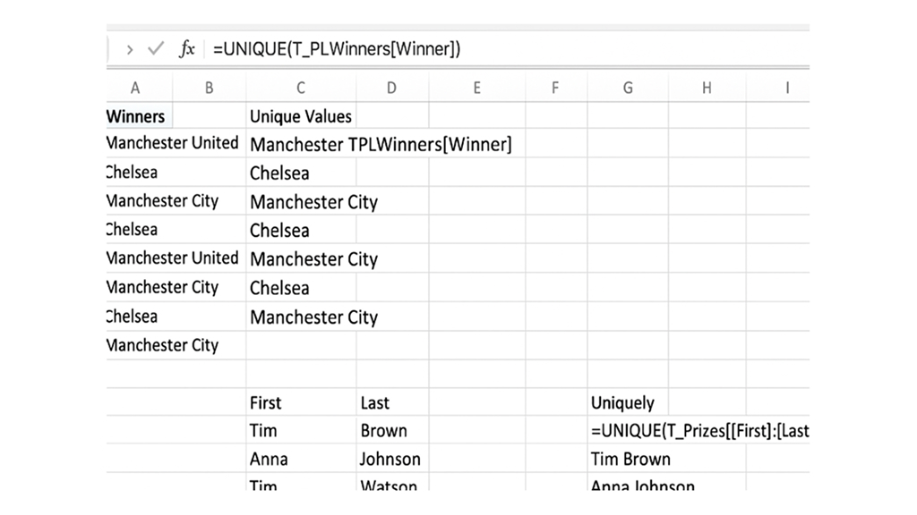
One of the most common uses of UNIQUE is to clean up a column that includes repeated entries. For example, consider a table named T_PLWinners that lists Premier League champions since 2010. Since some teams appear more than once, you can use UNIQUE to generate a clean list where each winner is listed only once. The function is also case-insensitive, meaning Winners, winners, and WINNERS are treated as the same text.
To extract a distinct list from the Winner column, enter the following formula in cell D2:
=UNIQUE(T_PLWinners[Winner])
Instead of typing the structured reference manually, you can select the entire column by hovering over the header until a small black arrow appears. Because you’re returning all unique items in that column, you don’t need to add arguments b or c. However, if the data were arranged horizontally across a row instead of down a column, you would set argument b to TRUE.
Since UNIQUE is a dynamic array function, the results automatically spill into the cells below and update whenever new rows are added to the source table.
Extracting Unique Values From Multiple Columns
When you’re working with datasets that involve multiple fields, such as Name, Department, and Location, you may need to extract unique combinations rather than unique values from a single column. This is especially useful when the same person may appear in different departments or offices, or when multiple employees share the same department but work in different locations. In such cases, Excel’s UNIQUE function becomes a powerful tool for generating a list of distinct multi-column entries.
Consider a dataset where each row contains an employee’s full details like Name, Department, and Location.
In the spreadsheet (as shown in the image), entries like Emily Jones – Marketing – Seattle or Michael Brown – Sales – New York may appear more than once or in varying combinations. Instead of manually filtering through each row, you can use the UNIQUE function to return only one instance of every unique combination across all selected columns.
To do this, simply reference the range that contains all the relevant columns. For example:
=UNIQUE(A2:C6)
Excel evaluates every row in the selected block and identifies full, distinct combinations. If two rows match across all referenced columns, only one will appear in the output. If even a single value differs, say the same employee appears in a different location—Excel treats it as a separate unique entry.
This method ensures:
- Cleaner datasets when working with employee lists or other multi-field records
- Accurate reporting, ensuring each unique combination is captured exactly once
- Dynamic results, automatically updating when new records are added
Using UNIQUE to Return Values That Appear Only Once

Sometimes you need to isolate items that occur just once, like one-time customers or products sold only once. Use:
=UNIQUE(A2:A200, , TRUE)
Using UNIQUE Alongside Other Excel Functions

This is where the real magic happens. UNIQUE becomes even more powerful when paired with other dynamic array functions.
1. COUNTA + UNIQUE
The combination of COUNTA and UNIQUE is one of the simplest yet most effective ways to count how many distinct values appear in a dataset. Instead of manually filtering duplicates or using complex formulas, this approach gives you an instant count of unique items using just two functions.
How It Works
- UNIQUE extracts all distinct values from a given range.
- COUNTA then counts how many items appear in the resulting unique list.
This two-step logic makes it easy to calculate unique entries in anything, names, product IDs, departments, cities, or any repetitive list.
Example
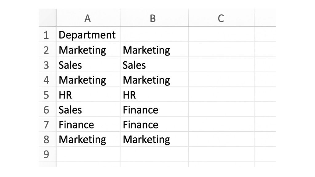
Imagine you have a list of employee departments in cells A1:A8
You can extract the unique departments using:
=UNIQUE(A1:A8)
This will return as Marketing, Sales, HR, and Finance. Now, to count how many unique departments exist, wrap UNIQUE inside COUNTA:
=COUNTA(UNIQUE(A1:A8))
The formula returns 4. This tells you there are four distinct departments in the list, regardless of how many times each one appears.
2. SORT + UNIQUE
The SORT and UNIQUE functions work brilliantly together when you need a list that is not only duplicate-free but also neatly arranged in alphabetical (or numerical) order. While UNIQUE removes repeated values, SORT organizes the remaining items so the output looks polished and easy to scan.
This combination is especially useful for tasks like preparing dropdown menus, generating clean reports, or quickly summarizing messy data.
Example
Imagine you have the following department list in cells A1:A8:
- Marketing
- Sales
- Marketing
- HR
- Sales
- Finance
- Finance
- Marketing
To create a sorted, duplicate-free department list, type this formula into B1:
=SORT(UNIQUE(A1:A8))
- UNIQUE pulls out only Marketing, Sales, HR, Finance
- SORT arranges them alphabetically; Finance, HR, Marketing, Sales
You end up with a clean, organized list ready for use anywhere—dropdowns, reporting dashboards, or analysis.
3. UNIQUE + FILTER
Sometimes you don’t want unique values from the entire dataset, you only want unique results that meet a specific condition. This is where combining UNIQUE with FILTER becomes incredibly powerful.
- The FILTER function first narrows down the data to only the rows that match your criteria.
- Then, UNIQUE removes duplicates from that filtered list.
Together, they help you extract meaningful, targeted insights from large or messy datasets.
Example:
If you have a list of employees with their names, departments, and locations, you can easily extract only the unique employees who belong to the Marketing department using the formula:
=UNIQUE(FILTER(A2:A7, B2:B7=”Marketing”))
In this scenario, the FILTER function first scans the Department column and pulls out only the names where the department is “Marketing,” giving you a filtered list containing John, Arjun, and Daniel. Once this shortened list is generated, the UNIQUE function takes over and removes any repeated names, ensuring that only distinct Marketing employees are returned.
The final result is a clean, duplicate-free list of Marketing team members, giving you an efficient way to segment and analyze your data without manually sorting through rows.
4. FILTER + UNIQUE + COUNTIF
The combination of FILTER + UNIQUE + COUNTIF is incredibly useful when you want to extract distinct values based on a condition and see how many times each of those values appears.
Imagine you have a list of customer names in column A and their purchase status (“Completed”, “Pending”, “Cancelled”, etc.) in column B. If you want to identify all the customers who have completed a purchase and calculate how many completed orders each one has, you can first use FILTER to pull only the rows marked “Completed.”
Next, when you apply UNIQUE to the filtered results, you get a clean list of unique customer names with completed purchases. Finally, COUNTIF is used alongside this list to count how many times each customer appears in the filtered data.
For example, imagine your filtered list includes the names Laura, Michael, Emma, and Laura. When the UNIQUE function is applied, it returns the distinct names Laura, Michael, and Emma. Next, COUNTIF checks how many times each name appears in the original filtered results, showing that Laura appears twice, while Michael and Emma appear only once.
=UNIQUE(FILTER(A2:A20, COUNTIF(A2:A20, A2:A20) > 1))
By combining FILTER, UNIQUE, and COUNTIF, you get a clear and efficient summary of your data, making it easy to spot duplicates and understand frequency patterns without doing any manual counting.
Everyday Use Cases for the UNIQUE Function in Excel

You’ll find UNIQUE extremely useful in all kinds of real-world data cleanup scenarios. Common practical uses are:
- Extracting unique product categories for inventory reporting
- Listing unique employee IDs in HR reports
- Summarizing unique city names from large sales data
- Cleaning email lists by removing repeated entries
- Identifying distinct regions, states, or segments in marketing data
- Removing duplicate responses in survey results
- Creating dropdowns that auto-update as new data arrives
The UNIQUE function is hands-down one of Excel’s most valuable modern tools. It makes data cleaning faster, smarter, and fully dynamic. Whether you’re extracting distinct values, isolating one-time entries, creating dropdown lists, or combining UNIQUE with SORT, FILTER, or COUNTIF, this function opens the door to powerful, automated spreadsheets.
If you regularly work with repeated entries, large datasets, or dynamic reports, mastering UNIQUE will make your Excel work dramatically easier. Once you get used to it, you’ll rely on it for everything from simple lists to advanced analyses.


